728x90
Keyframing and Splines
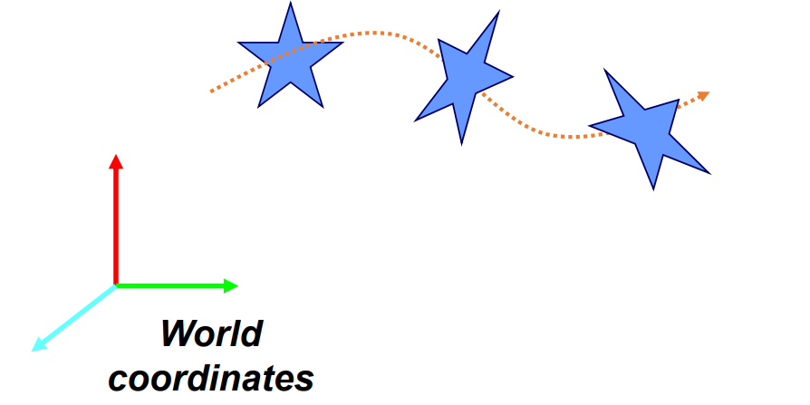
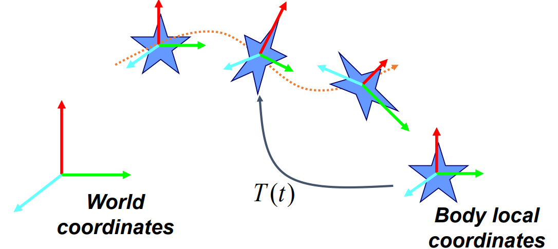
What is Motion?
- Motion is a time-varying transformation from body local system to world coordinate system. (in a very narrow sense)
Transformation
- Rigid Transformation(강체 변환)
- Rotate + Translate
- 3x3 orthogonal matrix + 3-vector
- $T : x → Rx + b$
- Affine Transformation(어파인 변환)
- Scale + Shear + Rigid Transformation
- 3x3 matrix + 3-vector
- $T: x → Ax + b$
- Homogeneous Transformation(동종 변환)
- Projective + Affine Transformation
- 4x4 homogeneous matrix
- $T: x → Hx$
- General Transformation(일반 변환)
- Free-form deformation
Keyframing

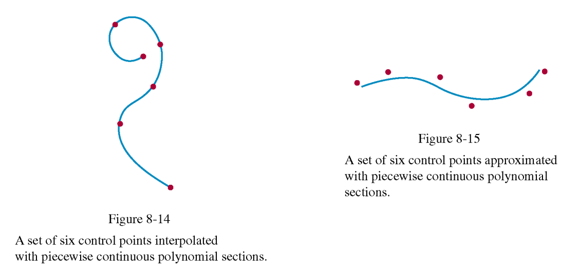
Interpolation and Approximation
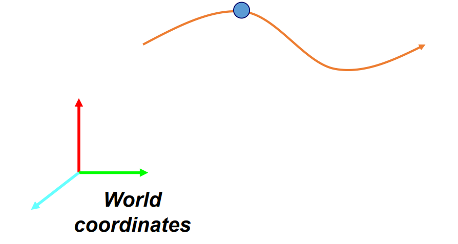
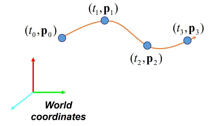
Particle Motion
- A curve in 3-dimensional space
- $p(t) = (x(t), y(t), z(t))$
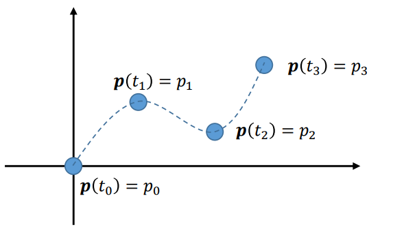
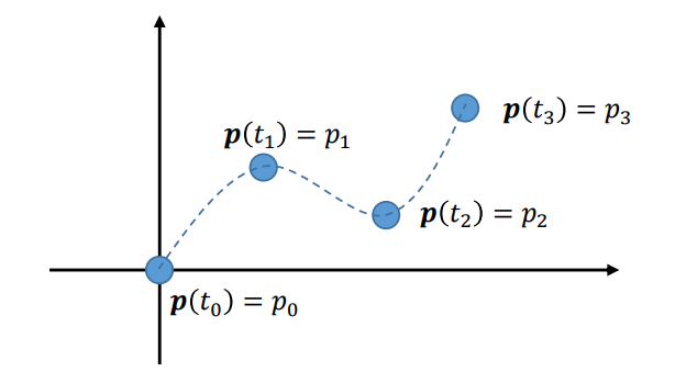
Keyframing Particle Motion
- Find a smooth function $p(t)$ that passes through given keyframes $(t_{i}, p_{i}), 0 ≤ i ≤ n$.
Polynomial Curve
- Mathematical Function vs. Discrete Samples
- Compact
- Resolution Independence
- Why Polynomials?
- Simple
- Efficient
- Easy to manipulate
- Historical Reasons
| $x(t) = a_{x}t^{3} + b_{x}t^{2} + c_{x}t + d_{x}$ $y(t) = a_{y}t^{3} + b_{y}t^{2} + c_{y}t + d_{y}$ or $z(t) = a_{z}t^{3} + b_{z}t^{2} + c_{z}t + d_{z}$ |
$p(t) = at^{3} + bt^{2} + ct + d$ |
Degree and Order
- Polynomial
- Order $n+1$ (= number of coefficients)
- Degree $n$
- $x(y) = a_{n}t^{n} + a_{n-1}t^{n-1} + \cdots + a_{1}t + a_{0}$
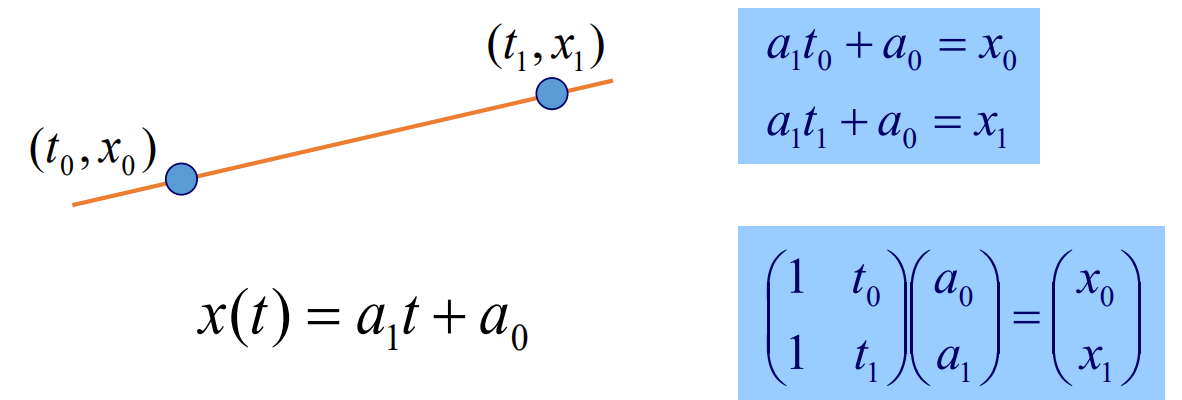
Polynomial Interpolation
- Linear Interpolation with a polynomial of degree one
- Input : Two Nodes
- Output : Linear Polynomial

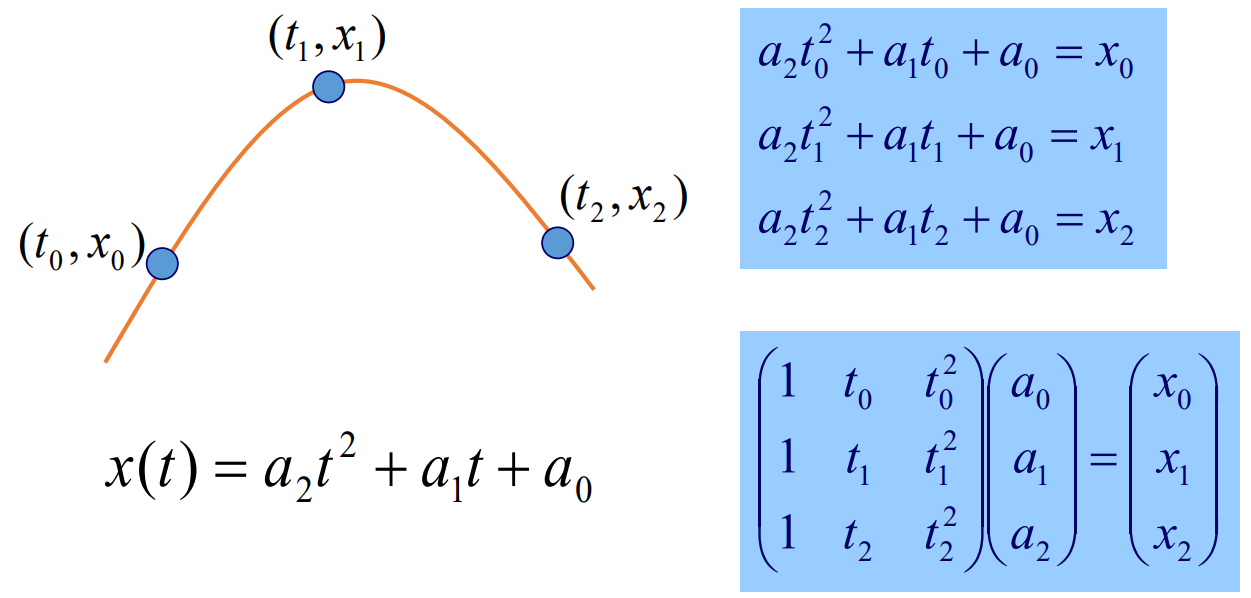
- Quadratic Interpolation with a polynomial of degree two
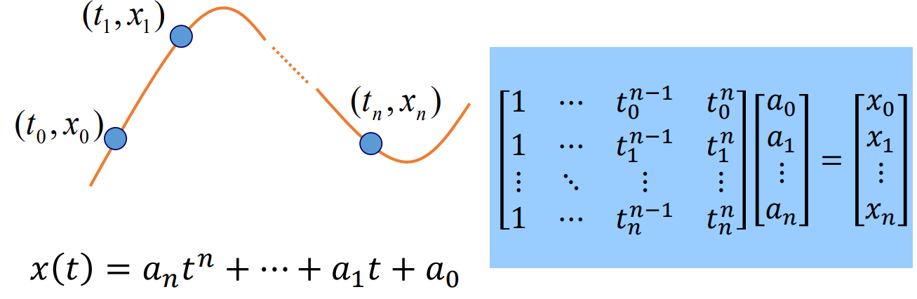
- Polynomial Interpolation of degree n
Do we really need to solve the linear system?
Question
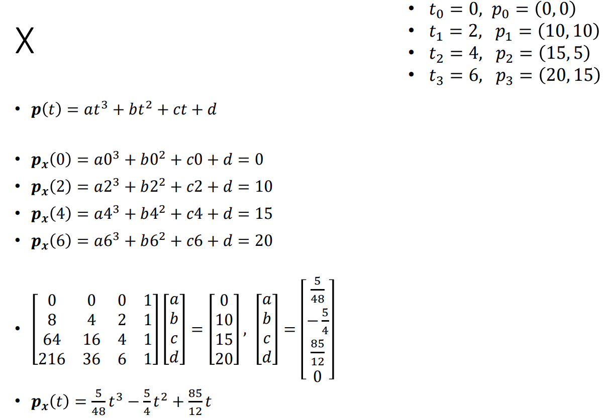
- Find a 4x4 matrix equation to solve for the polynomial, $p(t)$ interpolating the four key points.
- $p(t) = at^{3} + bt^{2} + ct + d$
- $t_{0} = 0, p_{0} = (0, 0)$
- $t_{1} = 2, p_{0} = (10, 10)$
- $t_{2} = 4, p_{0} = (15, 5)$
- $t_{3} = 5, p_{0} = (20, 15)$
Solution
 |
 |
Lagrange Polynomial(라그랑주 보간법)
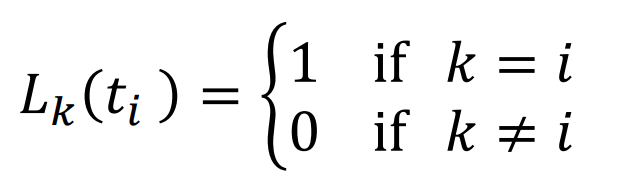
- Weighted sum of data points and cardinal functions
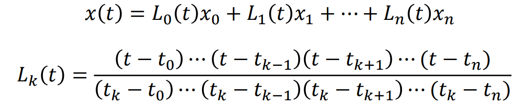
- Cardinal Polynomial Functions
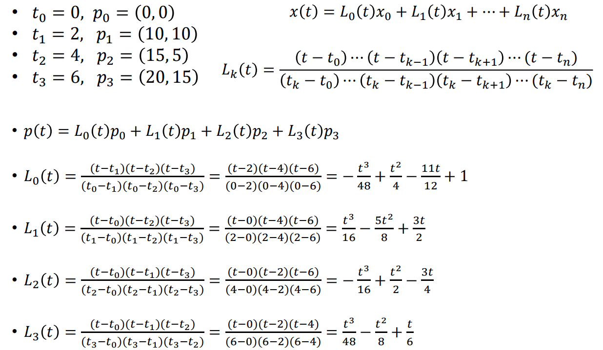
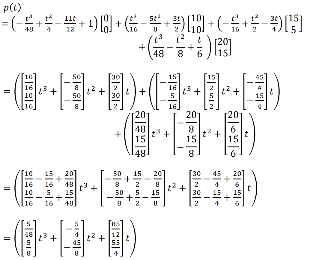
Question
- Find the Lagrange Polynomial Interpolating the four key points.
- $p(t) = L_{0}(t)p_{0} + L_{1}(t)p_{1} + L_{2}(t)p_{2} + L_{3}(t)p_{3}$
- $t_{0} = 0, p_{0} = (0, 0)$
- $t_{1} = 2, p_{0} = (10, 10)$
- $t_{2} = 4, p_{0} = (15, 5)$
- $t_{3} = 5, p_{0} = (20, 15)$
 |
 |
Limitation of Polynomial Interpolation
- Oscillations(진동, 움직임) at the ends
- Nobody uses higher-order polynomial interpolation now.
- Demo
Interpolating Lagrange curve
Interpolating Lagrange curve Interpolating curves are designed to run through all given points. The Bezier curve, for instance, goes through its endpoints only, because at the parameter values corresponding to the endpoints (t =0, t = 1) all the basis func
www.ibiblio.org
Spline
An Interactive Introduction to Splines
www.ibiblio.org
Splines
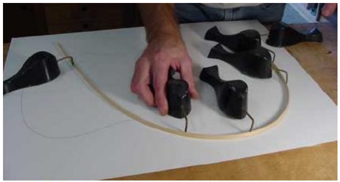
- Motivated by Loftman's Spline
- Long narrow strip of wood or plastic
- Shaped by lead weights (called ducks)
Simple Interpolation
- Piecewise smooth curves
- Low-degree (dubic for example) polynomials
- Uniform vs. Non-Uniform knot sequences
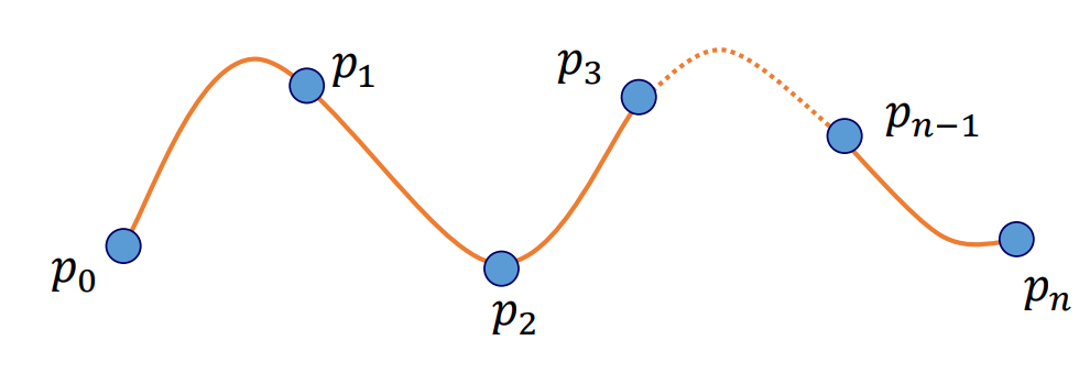
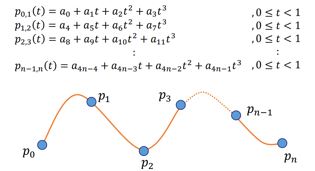
Cubic Splines
- Given $n+1$ key points, $n$ cubic polynomials are required.
- The knot points must be smoothly connected.
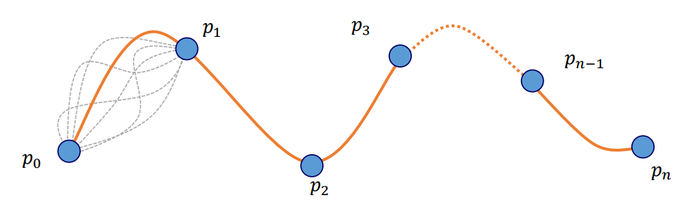
- There are infinitely many choices of cubic polynomials connecting given two points.
- Our goal is to choose cubic polynomials such that they are connected seamlessly at every knot points.
Why Cubic Polynomials?
- Cubic(degree of 3) polynomial is a lowest-degree polynomial representing a space value.
- Quadratic(degree of 2) polynomial is a planar curve.
- Eg). Front Design
- Higher-degree polynomials can introduce unwanted wiggles(꿈틀꿈틀한 움직임)
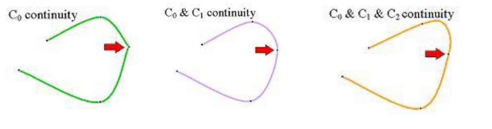
Parametric Continuity
- Zero-order parametric continuity
- $C^{0}$-continuity
- Means simply that the curves meet.
- First-order parametric continuity
- $C^{1}$-continuity
- The first derivatives(도함수) of two adjoining curve functions are equal.
- Second-order parametric continuity
- $C^{2}$-continuity
- Both the first and the second derivatives of two adjoining curve functions are equal.
Splines
- Catmull-Rom Spline
- Natural Cubic Spline
- B-Spline
728x90
'Computer Graphics' 카테고리의 다른 글
| [Computer Animation] B-Spline (0) | 2022.05.01 |
|---|---|
| [Computer Animation] Natural Cubic Spline (0) | 2022.05.01 |
| [Computer Animation] Catmull-Rom Spline (0) | 2022.05.01 |
| [Computer Animation] Bezier Curve & Bezier Spline (0) | 2022.05.01 |
| [Unreal Engine 4] 블루프린트 클래스(Blueprint Class)에 Static Mesh 연결하기 (0) | 2022.04.24 |
| [Unreal Engine 4] 새로운 월드 생성 & 기본 환경 설정 (0) | 2022.04.16 |
| [Computer Animation] Slerp(Spherical Linear Interpolation) (0) | 2022.04.10 |
| [Computer Animation] 3D Rotation and Orientation (0) | 2022.04.10 |